
The article develops a mathematical model for one-dimensional gravity-capillary ship waves, using residue theory to analyze wave components and show how surface tension and wave number differences influence the formation of sinusoidal wave patterns.
Consider 1-D gravity-capillary waves, the surface displacement is described by: \[ \begin{equation} \frac{2 \pi \eta}{P}=\lim _{\epsilon \rightarrow 0}\left\{\int_0^{\infty} \frac{e^{i k x_1} d k}{k U^2-2 i \epsilon U-g-(T / \rho) k^2}+\int_0^{\infty} \frac{e^{-i k x_1} d k}{k U^2+2 i \epsilon U-g-(T / \rho) k^2}\right\} . \end{equation} \] The above integral is divided into two parts, which are defined as: \[ \begin{equation} \begin{aligned} & J_1=\int_0^{\infty} \frac{e^{i k x}}{k U^2-2 i \epsilon U-g-\frac{T}{\rho} k^2} d k \\ & J_2=\int_0^{\infty} \frac{e^{-i k x}}{k U^2+2 i \epsilon U-g-\frac{T}{\rho} k^2} d k \end{aligned} \end{equation} \] The equation \((2)\) can be solved based on the residue theorem, for \(J_1\),it is readily apparent that it has two poles, \(k_g+i\xi\) and \(k_T+i\xi\). Subsequently, we employ Taylor series expansion to determine \(\xi\), firstly, we put \[ \begin{equation} I_1=kU^2-g-\frac{T}{\rho}k^2 \end{equation} \] It follows that \[ \begin{equation} I_1(k_g)=0; \quad I_1(k_T)=0 \end{equation} \] We expand the function \(I_1\) in a Taylor series about \(k_0(k_T\text{ or }k_g)\) \[ \begin{equation} I_1(k)=I_1\left(k_0\right)+I^{\prime}\left(k_0\right)\left(k-k_0\right) \end{equation} \]
It follows that
\[ I_1\left(k_0+i \xi\right)=I_1\left(k_0\right)+I^{\prime}\left(k_0\right) i \xi \]
Subsequently, we posit \(I_2\) as
\[ \begin{aligned} I_2(k) & =k U^2 - 2 i\epsilon U-g-\frac{T}{\rho} k^2 \\ & =I_1(k) - 2 i \epsilon U \end{aligned} \]
Based on assumption. we know that \(k_0+i \xi\) is the root of \(I_2=0\), then \[ \begin{equation} \begin{aligned} I_2\left(k_0+i \xi\right) & =I_1\left(k_0+i \xi\right) - 2 i \epsilon U \\ & =\underbrace{I_1\left(k_0\right)}_0+I^{\prime}\left(k_0\right) i \xi - 2 i \epsilon U \quad(=0) \end{aligned} \end{equation} \] therefore
\[ \begin{equation} I^{\prime}\left(k_0\right) i \xi - 2 i \epsilon U=0 \end{equation} \]
we have
\[ \begin{aligned} I^{\prime}(k) & =u^2-\frac{2 T}{\rho} k \\ \Rightarrow \quad I^{\prime}\left(k_0\right) & =u^2-\frac{2 T}{\rho} k_0 \end{aligned} \]
finally
\[ \begin{equation} \xi=\frac{2 i \epsilon U}{U^2-\frac{2 T}{\rho} k_0} \end{equation} \] for \(k_g\) consider the denominator of \(\xi\)
\[ u^2-\frac{2 T}{\rho} k_0=u^2-\frac{2T}{\rho} k_g \]
and we have
\[ \Rightarrow \quad \begin{gathered} k_g u^2-g-\frac{T}{\rho} k_g^2=0 \\ \quad U^2=\frac{g}{k_g}+\frac{T}{\rho} k_g \end{gathered} \]
there fore
\[ \begin{equation} \begin{aligned} U^2-\frac{2 T}{\rho} k_g & =\frac{g}{k_g}+\frac{T}{\rho} k_g-\frac{2 T}{\rho} k_g \\ & =\frac{g}{k_g}-\frac{T}{\rho} k_g \end{aligned} \end{equation} \] from equation \((3)\) \[ \begin{aligned} & k_T k_g=\frac{p g}{T} \\ \Rightarrow \quad & \frac{g}{k_g}=\frac{T}{\rho} k_T \end{aligned} \]
then eqn \((9)\) becomes
\[ \begin{aligned} U^2-\frac{2 T}{\rho} k_g & =\frac{T}{\rho} k_T-\frac{T}{\rho} k_g \\ & =\frac{T}{\rho}\left(k_T-k_g\right) \end{aligned} \] Hence, for a root of \(k_g\), the associated value of \(\xi\) is: \[ \begin{equation} \xi=\frac{2 \epsilon \rho U}{T\left(k_T-k_g\right)} i \end{equation} \] Similarly, for a root of \(k_T\), \(\xi\) denotes \[ \begin{equation} \xi=-\frac{2 \epsilon \rho U}{T\left(k_T-k_g\right)} i \end{equation} \] Applying residue theorem (for \(J_1\)), we obtain \[ \begin{equation} \eta=2 \pi i \sum_{i=1}^n \operatorname{Res}\left[f(k), k_i\right] \cdot \frac{p}{2 \pi} \end{equation} \] Concerning gravitational capillary waves, the poles are respectively
\[ k_{0, g}=k_g+\frac{2 \rho U}{\left(k_T-k_g\right) T}i \epsilon; \quad k_{0, T}=k_T-\frac{2 \rho U}{\left(k_T-k_g\right) T} i\epsilon \]
To ensure the integrability of the integrand, it's necessary that (Jordan's Lemma) \[ \Re[i k x]<0 \]
therefore
\[ \Im[k x]>0 \]
now, we consider \(x>0\), then
\[ \Im[k]>0 \] thus the pole is
\[ k_{0, g}=k_g+\frac{2 \rho U}{\left(k_T-k_g\right) T} i \epsilon \] Conversely, as \(x<0\) the pole is \[ k_{0,T}=k_T+\frac{2\rho U}{T\left(k_T-k_g\right)}i\epsilon \]
Appendix: Jordan's Lemma
we use Jordan's Lemma. Its form
\[ \int_{-\infty}^{\infty} f(k) e^{i k x} d k \]
we want to integrate a function of the form over a contour in the complex plane. Specifically, consider a large semicircle in either the upper or lower half plane (depending on the sign of \(x\) ) of Radius \(R\). Jordan's Lemma says:
if \(f(k)\) is well-behaved (eg. bounded or goes to zero sufficiently fast on that semicircle of radius \(R\)), and if the exponential factor \(e^{ikx}\) exhibits exponential decay on that arc (ie. \(\Im(k)>0\)) so that the imaginary part of the exponent is negative then \[ \lim _{R \rightarrow \infty} \int_{\text {Semicircle }} f(k) e^{i k x} d k=0 \] like:
\[ \oint_c f(k) d k=\int_{-R}^R f(k) d k+\int_{\text {arc }} f(k) d k \]
and applying the residue theorem, we find that
\[ \oint_c f(k) d k=2 \pi i \sum_{i=1}^n \operatorname{Res}\left[f(k), k_i\right] \]
Clearly, according to Jordan's theorem, we have
\[ \begin{aligned} & \int_{\operatorname{arc}} F(k) d k=0 \\ \Rightarrow & \oint_c F(k) d k=\int_{-R}^R F(k) d k \end{aligned} \]
Now consider our case, since the term \(e^{i k x}\), then in the case where \(x>0\), corresponding to \(k_0 \rightarrow k_g\). \(\Re[i k x]\) must be negative according to Jordan's Lemma, therefore
\[ \Im[k]>0 \text { for } k_0=k_g \]
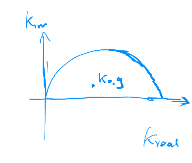
As illustrated in the figure
Applying the residue theorem. for \(k_{0, g}\) \[ \operatorname{Res}\left[k_0\right]=\lim _{k-k_i}\left(k-k_i\right) f\left(k_i\right) \]
Note that:
\[ \oint f(z) d z=2 \pi i \sum_{i=1}^n \operatorname{Res}\left[f(z), z_i\right] \]
when \(x>0 \quad\left(\epsilon \rightarrow 0\right)\) the component related to the pole \(k_{0, g} \rightarrow k_g\)
\[ \begin{aligned} J_{1,g} & =i p \lim _{k \rightarrow k_{g}}\left(k-k_g\right) \frac{e^{i k_g x}}{\frac{T}{\rho}\left(k-k_g\right)\left(k-k_T\right)} \\ & =-i \frac{p \rho}{T} \frac{e^{i k_g x}}{k_g-k_T} \\ & =i \frac{p \rho}{T} \frac{e^{i k_g x}}{k_T-k_g} \\ & =i \frac{\rho p}{T\left(k_T-k_g\right)}\left(\cos k_g x+i \sin k_g x\right) \\ & =-\frac{\rho p}{T\left(k_T-k_g\right)} \sin k_g x, \quad\text{(real part)} \end{aligned} \]
Subsequently, we consider the component of \(J_2\) related to gravity waves (the part \(x>0\)), and the pole are
\[ k_{0, g}=k_g-\frac{2 \rho U}{\left(k_T-k_g\right) T}i\epsilon; \quad k_{0, T}=k_T+\frac{2\rho U}{\left(k_T-k_g\right) T} i\epsilon \]
and
\[ \begin{aligned} J_{2,g} & =i p \lim _{k \rightarrow k_g}\left(k-k_g\right) \frac{e^{-i k_g x}}{\frac{T}{\rho}\left(k-k_g\right)\left(k-k_T\right)} \\ & =i p \frac{\rho}{T\left(k_g-k_T\right)} e^{-i k_g x} \\ & =-i\frac{\rho p}{T\left(k_T-k_g\right)}\left(\cos k_g x-i \sin k_g x\right) \\ & =-\frac{\rho P}{T\left(k_T-k_g\right)} \sin k_g x, \quad\text{(real part)} \end{aligned} \]
confining the two above, we have the gravity component \(\eta_{g}\) (\(x>0\)),
\[ \eta_g=-\frac{2 \rho p}{T\left(k_T-k_g\right)} \sin k_g x \]